- Research
- Open access
- Published:
Reachability-based model reduction for Markov decision process
Journal of the Brazilian Computer Society volume 21, Article number: 5 (2015)
Abstract
This paper presents how to improve model reduction for Markov decision process (MDP), a technique that generates equivalent MDPs that can be smaller than the original MDP. In order to improve the current state-of-the-art, we take advantage of the information about the initial state of the environment. Given this initial state information, we perform a reachability analysis and then employ model reduction techniques to the reachable space of the original problem. Further, we also eliminate redundancies in the original MDP in order to speed up the model reduction phase. We also contribute by empirically comparing our technique against state-of-the-art model reduction techniques and MDP solvers that do not perform model reduction. The results show that our approach dominates the current model reduction algorithms and outperforms general MDP solvers in dense problems, i.e., problems in which actions have many probabilistic outcomes.
Background
One of the biggest challenges in the probabilistic planning is to solve large Markov decision processes (MDPs) [1]. This is because the number of states in an MDP grows exponentially with the number of state variables, a problem known as the Bellman’s curse of dimensionality [1]. Many techniques have been proposed to avoid the complete enumeration of states, e.g., by exploiting the structure of factored models [2, 3] and by using the information of the initial state to find the states relevant for the optimal solution by focusing on them [4, 5].
Another approach is to apply model reduction to obtain a smaller MDP and then solve it using an off-the-shelf MDP solver [6]. In order to find the optimal solution for the original MDP, both the original and reduced MDP must be equivalent. Therefore, the problem of finding an equivalent and reduced MDP consists of computing a partition \(\mathcal {P}\) of the original MDP state space S, such that each block represents a subset B i ⊆S that groups equivalent states according to their reward and probabilistic transition functions.
This paper extends the algorithms for computing stochastic bisimulation in two directions: reachability analysis and partition elimination. In the former, we use the MDP’s initial state to find all the states relevant to the optimal solution and consider only this subspace of the original problem when applying model reduction. In the latter, we detect and delete intermediary partitions of the original MDP that are repeated, thus speeding up the convergence to a stochastic bisimulation. We also contribute with an empirical comparison among: the state-of-the-art model reduction algorithms and MDP solvers (that do not perform model reduction). The results show that our approach dominates the current model reduction algorithms in all problems, specially in sparse domain problems where reachability analysis prunes a significant part of the state space. The experiments also show that our technique outperforms general MDPs solvers (that do not perform model reduction) in dense problems, i.e., problems in which actions have many probabilistic outcomes. This is true specially when the domain suffer a significant reduction. This happens because stochastic bisimulations with partition elimination can summarize the dynamics of the domain and generate equivalent problems with half of the original MDP size.
The paper is organized as follows. The “Background” section presents our notation, background related to MDPs, and algorithms to solve them. The “Aggregation algorithms” section presents the concepts of state aggregation algorithms and stochastic bisimulation, as well as the basic algorithm to compute them. The “Stochastic bisimulation over the reachable states” section contains our contributions to algorithms that compute stochastic bisimulations. The section “Results and discussion” empirically compares our technique combined with traditional planners against traditional model reduction algorithms and planners that do not employ model reduction. Finally, the “Conclusions” section presents our conclusions.
Markov decision processes
An infinite-horizon MDP [1] is a tuple M=(S,A,P,R,γ), where:
-
S is a finite set of states that can be observed in different moments in time;
-
A is a finite set of actions and A(s)⊆A is the set of applicable actions in the state s;
-
P:S×A×S is the transition function and is given by P(s ′|s,a) that defines the probability to reach s ′∈S after applying an action a∈A in s∈S. P(·|·,a) defines a probabilistic transition matrix where each row represents a state s, each column represents a state s ′ and an entry (s,s ′) has the probability P(s ′|s,a). We say that the transition matrix is dense if at least 50 % of the entries have probabilities greater than 0; otherwise, we called it a sparse transition matrix;
-
R:S×A is the reward function that represents the reward received after applying an action a∈A in the state s∈S; and
-
γ∈]0,1[ is the discount factor used for weighting future rewards [1].
A solution of an MDP is a policy π:S↦A that maps each state s∈S to an action a∈A.
The expected accumulated reward obtained when following a policy π from a state s is represented as V π(s) and is the fixed-point solution for the following system of equations:
A policy π ∗ is optimal if, for every policy π ′ and s∈S, \(V^{\pi '}(s) \le V^{\pi ^{*}}(s)\phantom {\dot {i}\!}\). Notice that π ∗ might not be unique; however, the optimal expected accumulated reward from a state s, denoted by V ∗(s), is unique [7]. The value function V ∗ can be computed directly by finding the fixed-point solution of the Bellman equations, i.e., the following system of equations:
An MDP M=(S,A,P,R,γ) is enumerative if all elements of all sets that constitute the MDP are explicitly enumerated, e.g., state space S and probability tables P are represented directly by enumerating each element of them. Alternatively, an MDP can be represented in a factored form based on a set of state variables X={X 1,…,X n }. Each state is represented as a vector \(\vec {x} = (x_{1},\ldots,x_{n})\) of assignments where each x i is either 0 or 1 to denote if the state variable X i is active or not. Thus, the size of the set of states in a factored MDP is 2n.
The transition function of a factored MDP is represented by a set of dynamic Bayesian networks (DBNs) [8], one for each action. A DBN for an action a is an acyclic directed graph that has the following two layers: (i) a layer representing the set X of state variables in the current state and (ii) a layer representing the set X ′ of state variables in the next state. Every arc in a DBN representing an action is from the layer X to X ′ and represents the dependencies between state variables under an action a. Given a variable X j′, the parents of X j′ (denoted by parents(X j′)) are all variable X i such that there exists an arc from X i to X j′.
A DBN also contains the conditional probability tables (CPTs) that give us the probability of a state variable X j′ being true or false given the parents of X j′. The advantage of using DBNs is that we do not need to enumerate all possible combinations of state variable values to represent the transition function. Instead, it is obtained as follows:
An efficient way to represent the CPTs (and factored reward functions) is through algebraic decision diagram (ADD) [9]. ADDs extend binary decision diagrams (BDDs) [10]. BDDs are decision trees represented in a more compact way in order to efficiently define functions with binary variables to a binary result, i.e., \(f: \mathbb {B}^{n} \mapsto \mathbb {B}\). ADDs are used to represent functions that map binary variables to real values, i.e., \(f:\mathbb {B}^{n} \mapsto \mathbb {R}\). Thus, to solve an MDP, we can also represent the value function as an ADD. There are ADD libraries to efficiently compute operations such as addition (⊕), multiplication (⊗), and marginalization \(\left (\sum _{x_{i} \in X_{i}}\right)\).
Algorithms for solving MDPs
Value iteration and topological value iteration
The value iteration (VI) algorithm [1] uses dynamic programming in order to find V ∗. Formally, VI solves the following recursive equations, where t is the number of stages-to-go:
The algorithm converges to V ∗ when the maximum error between the last two iterations is less than a small constant ε, for all state s∈S. This is expressed as:
VI can take a long time to converge because it needs to update the values of the complete set of states S in each iteration independently of the problem structure.
Topological value iteration (TVI) [11], an extension of VI, exploits the topological structure of the transition graph to speed up the convergence time by decreasing the number of updates performed.
Formally, TVI pre-processes the given MDP by performing a topological analysis of the graph representing the MDP, i.e., a graph in which the nodes are states and the arcs are actions. The result of this analysis is a set of the strongly connected components (SCCs) and TVI applies VI on each SCC in reversed topological order. This decomposition can speed up the convergence to V ∗ when the original MDP can be decomposed into several SCCs with similar size. In the worst case, when the MDP has only one SCC, TVI performs worst than VI due to the overhead of the topological analysis.
Labeled real-time dynamic programming
Stochastic shortest path problem (SSP) [7] is another model for probabilistic planning. The main differences between SSPs and infinite-horizon MDPs is that SSPs contain the information about the initial state of the environment as well as a set of goal states representing the stop criterion of the agent. Formally, an SSP is a tuple (S,s 0,G,A,P,C) where:
-
as in the MDPs, S, A, and P are the set of states, set of actions, and transition function respectively;
-
s 0∈S is the initial state;
-
G⊂S is the non-empty set of goal states; and
-
C:S×A represents the cost of applying action a∈A in the state s∈S.
SSPs are relevant for this work because any infinite-horizon MDP can be perfectly represented as an SSP [12, Section 7.3], thus we can also use algorithms developed for SSPs to solve the problems presented in this paper.
One example of algorithm for solving SSPs is real-time dynamic programming (RTDP) [4] that, given an SSP and a lower bound for V ∗, computes an optimal policy for all the relevant states, i.e., all states reachable by the optimal policy starting from s 0. RTDP starts from s 0 and visits the set of states following a greedy policy until a goal state is reached. This procedure is known as a trial and, for the case of infinite-horizon MDPs converted to SSPs, a trial can be seen as an infinite process that randomly finishes with probability 1−γ every time a state is visited. RTDP performs trials until it has converged to the optimal solution.
In each state s visited in a trial, RTDP computes the greedy policy in s (the action that maximizes Equation 4), updates V t(s), and samples a next state to be visited based on the probability distribution of the greedy action. Due to this sampling procedure, states with a low probability are updated less often than states with a higher probability, resulting in overall lower convergence.
Labeled RTDP (LRTDP) [5] is an algorithm that enhances RTDP providing a faster convergence of the optimal solution. This performance improvement is obtained by labeling the states that have already converged and finishes the trials when a converged state or goal is reached. LRTDP uses the procedure CheckSolved [5] that is responsible to decide if a state is converged or not. This decision is done based on the concept of greedy graph of a state s, i.e., the graph that contains all reachable states from s following the greedy policy. The optimal solution is obtained when all states in the greedy graph of s 0 are marked as converged.
Aggregation algorithms
Given an MDP M, an optimal policy for M can be found by using VI, TVI, or LRTDP. Another way to find an optimal policy is based on two steps: (1) getting an equivalent model of reduced size based on the original MDP and (2) solving the reduced model and applying the solution in the original MDP. The first step is known as state aggregation for MDPs [13].
Mathematically, state aggregation algorithms for MDPs receive as input an MDP M=(S,A,P,R,γ) and computes a reduced MDP M ′=(S ′,A,P ′,R ′,γ) with a set of states S ′ that groups states into blocks of states, called abstract states in M ′. It is desirable that: the set of states of M ′ be much smaller than the set of states of M, i.e., |S ′|≪|S| and an optimal solution for M ′ to also be optimal for M.
There are many techniques for MDPs in the state aggregation category. For example:
-
Stochastic bisimulations (exact/approximate) [6, 14], a technique that receives an MDP (factored or enumerative) and returns an enumerative MDP (or a bounded-parameter MDP [15], i.e., an MDP whose functions are given by intervals);
-
Homomorphisms (exact/approximate) [16, 17], techniques that are similar to stochastic bisimulations, but can achieve greater reductions in some special scenarios;
-
Structured policy iteration (SPI) [18], one of the first techniques to use decision trees to solve factored MDPs;
-
Stochastic planning using decision diagrams (SPUDD) [2], a technique that is a factored version of value iteration. This was the first algorithm that used ADDs to solve MDPs more efficiently; and
-
Symbolic real-time dynamic programming - sRTDP [3], a factored version of RTDP that also uses decision diagrams.
A complete overview about state aggregation algorithms is presented in [13]. Some of these algorithms are completely factored, that is, they never use the concept of enumerative states set. At the same time, others can combine factored and enumerative representations. We chose exact stochastic bisimulations because with them, we can easily compare time and reduction performance against exact enumerative MDP planners. Moreover, we do not need to define a criterion to compare different approximate solutions because the exact solutions are unique. Thus, from now on, we will consider that model reduction and model minimization are algorithms that compute exact stochastic bisimulations.
The state aggregation algorithms for MDPs usually work based on the concept of partitions. A partition of a set S is a set of disjoint subsets whose union is S itself. Each disjoint subset can also be called a block. Given an enumerative MDP M and a set of states S, a partition over S is given by \(\mathcal {P} = \{B_{1}, \ldots, B_{k}\}\), where \(\mathcal {P}\) is a partition of S and each B i ∈{1,…,k} is a block.
Two important concepts for model reduction are refinement and coarsening of a partition. A partition \(\mathcal {P}'\) is a refinement of a partition \(\mathcal {P}\) if and only if each block of \(\mathcal {P}'\) is a subset of some block in \(\mathcal {P}\), i.e., a refinement splits a block B i in sub-blocks generating a finer partition. If \(\mathcal {P}' = \mathcal {P}\), \(\mathcal {P}'\) still is a refinement of \(\mathcal {P}\). The concept of coarsening is opposite to the concept of refinement: if \(\mathcal {P}'\) is a refinement of \(\mathcal {P}\), \(\mathcal {P}\) is a coarsening of \(\mathcal {P}'\) [6].
Definition 1.
Given that \(\mathcal {P}_{1}\) and \(\mathcal {P}_{2}\) are partitions of S described by enumerative states, we can generate a partition \(\mathcal {P}_{3}\) that is a refinement of \(\mathcal {P}_{1}\) and \(\mathcal {P}_{2}\) with the intersection of them, i.e., \(\mathcal {P}_{3} = \mathcal {P}_{1} \cap \mathcal {P}_{2}\) such that each \(B_{k} \in \mathcal {P}_{3}\) is computed by the intersection of two blocks \(B_{i} \in \mathcal {P}_{1}\) and \(B_{j} \in \mathcal {P}_{2}\), with B i ∩B j ≠∅. To compute every \(B_{k} \in \mathcal {P}_{3}\), it is necessary to do all combinations of B i ∩B j .
If we use factored representation instead of enumerative representation, it is possible to get more efficient algorithms for performing model reduction [6]. Hence, let X={X 1,…,X n } be the set of state variables of a given factored MDP and S⊆2n a set of valid states of this MDP. A block of states can be characterized by a disjunctive normal form (DNF) expression over the boolean variables in X, i.e., B i can be represented as a boolean formula and we use a label v i to identify the block. Thus, a labeled partition of S is a set \(\mathcal {P} = \{(B_{1}, v_{1}), \ldots, (B_{k}, v_{k})\}\) such that (\(\bigcup _{i=1}^{k} B_{i}) = S\). Furthermore, as \(\mathcal {P}\) is a an augmented partition, each pair v i ,v j associated with blocks B i ,B j must be different and unique in the partition. Each \((B_{i}, v_{i}) \in \mathcal {P}\) is a tuple with a partition block B i and an unique label v i that is common to all s∈B i . For instance, \(\mathcal {P} = \{(X_{1}, 2), (\neg X_{1}, 3)\}\) is a labeled partition with two blocks: a block of states, labeled with 2, where X 1 is satisfied and a block of states, labeled with 3, where ¬X 1 is satisfied.
Definition 2.
Given that \(\mathcal {P}_{1}\) and \(\mathcal {P}_{2}\) are labeled partitions of S described by DNF expressions, we can generate a partition \(\mathcal {P}_{3}\) that is a refinement of \(\mathcal {P}_{1}\) and \(\mathcal {P}_{2}\) with the intersection of them, i.e., \(\mathcal {P}_{3} = \mathcal {P}_{1} \cap \mathcal {P}_{2}\) where \(B_{k} \in \mathcal {P}_{3}\) is computed by the conjunction (∧) of two blocks \(B_{i} \in \mathcal {P}_{1}\), \(B_{j} \in \mathcal {P}_{2}\) such that B i and B j are not mutually exclusive DNF expressions of the kind X 1∧¬X 1. To compute every \(B_{k} \in \mathcal {P}_{3}\), it is necessary to compute all combinations of conjunctions considering different possibilities of B i ∩B j . The label v k must be different from the labels v i and v j . By definition, a partition of S with a single block is represented by the boolean expression true.
For example, given the partitions (Fig. 1) \(\mathcal {P}_{1} = \{(X_{1}, 2),(\neg X_{1}, 3)\}\) and \(\mathcal {P}_{2} = \{(X_{2} \land X_{3}, 5), (X_{2} \land \neg X_{3}, 7),(\neg X_{2}, 11)\}\), their intersection will result in the refined partition \(\mathcal {P}_{3} = \{(X_{1} \land X_{2} \land X_{3}, 10)\), (X 1∧X 2∧¬X 3,14), (X 1∧¬X 2,22), (¬X 1∧X 2∧X 3,15), (¬X 1∧X 2∧¬X 3,21), (¬X 1∧¬X 2,33)}. In general, given m partitions \(\mathcal {P}_{1}\), …, \(\mathcal {P}_{m}\), it is possible to get a refinement by computing the intersection of them as \(\mathcal {P}' = \bigcap _{i=1}^{m} \mathcal {P}_{i}\) [6].

Refinement of partitions. Refinement of partitions \(\mathcal {P}_{1}\) with two blocks and \(\mathcal {P}_{2}\), with three blocks. The refinement result is given by \(\mathcal {P}_{1} \cap \mathcal {P}_{2}\), a partition with six blocks
Figure 2 shows a sequence of refinements. In the beginning of the first iteration, it is given a partition with a single block. After the first iteration of refinements, the partition is split into two blocks. In the next two iterations, we get partitions of two and three blocks, respectively. Finally, a new refinement is done and the partition does not change. Hence, it is not necessary to split more blocks. From this example, we could extract an MDP M ′ with |S ′|=5.

A sequence of refinements. A partition with one block is refined until it reaches five blocks. Note that each refinement imply in a new partition that have at least the same number of blocks
Given a factored MDP, it is possible to use its reward and transition functions to identify blocks of states with the same reward or transition probability. For example, consider the domain Sysadmin, where we have n computers that must be running. Given a problem (instance) of this domain, we can apply the actions rebootC i or n o o p at each stage of the MDP. In an instance with two computers: C1 and C2, we have two state variables: runningC1 and runningC2 and three actions: n o o p, rebootC1 and rebootC2. The reward function for the action n o o p, given as an ADD, can be viewed in Fig. 3. For instance, if we execute the n o o p action in the state where runningC1 is true and runningC2 is false, the reward is 1. To refer to the partitions of an MDP, we use a special notation: for each action a∈A, we have a partition \(\mathcal {P}_{R}^{a}\) with respect to the reward function; and for each pair of action a∈A and state variable X i ∈X that can be changed by a, we have a partition \(\mathcal {P}_{X_{i}}^{a}\) with respect to the factored probabilistic transition function.

Reward function as a table. Reward function for action noop in an instance of the domain SysAdmin with 2 computers
The partition obtained from the reward function in Fig. 4 is implicitly represented as \(\mathcal {P}_{R}^{\text {noop}} = \{(B_{1},v_{1}), (B_{2},v_{2}), (B_{3},v_{3})\}\), where: B 1={runningC1∧runningC2}, with reward 2; B 2={(¬runningC1∧runningC2)∨(runningC1∧¬runningC2)}, with reward 1; and B 3={¬runningC1∧¬runningC2}, with reward 0. We can do the same for the other actions generating the partitions: \(P_{R}^{\text {reboot}C1}\) and \(P_{R}^{\text {reboot}C2}\).

Reward function represented as an ADD. The same reward function from Fig. 3 represented as an ADD
The partitions obtained from the factored probabilistic transition functions, for the Sysadmin example, for each pair of action and state variable are: \(\mathcal {P}_{\text {running}C1}^{\text {noop}}\), \(\mathcal {P}_{\text {running}C2}^{\text {noop}}\), \(\mathcal {P}_{\text {running}C1}^{\text {reboot}C1}\), \(\mathcal {P}_{\text {running}C2}^{\text {reboot}C1}\), \(\mathcal {P}_{\text {running}C1}^{\text {reboot}C2}\) and \(\mathcal {P}_{\text {running}C2}^{\text {reboot}C2}\). Thus, in general, the maximum number of different partitions we can have is |A|+(|A|×|X|), where |A| comes from the reward function of each action and |A|×|X| comes from the factored probabilistic transition functions considering each pair of action and state variable.
A labeled partition can be represented using an ADD where each leaf represents an unique label v i . The DNF expression that characterizes a block of states B i is given by the disjunction of the conjunctions among state variables, obtained from different paths that go from the ADD root to the leaf labeled with v i . For instance, Fig. 5 shows an ADD that represents the following labeled partition:

A partition represented as an ADD and its DNF expression. A partition \(\mathcal {P}\) of a set of states S in which the blocks are represented by the set of state variables X={X 1,X 2}. The partition is \(\mathcal {P} = \{(X_{1} \wedge X_{2}, 2), ((X_{1} \wedge \neg X_{2}) \vee (\neg X_{1} \wedge \neg X_{2}), 3), (\neg X_{1} \wedge X_{2}, 5)\}\)
To compute the refinement of q labeled partitions represented as ADDs, we need to get the product of ADDs representing these partitions. Note that performing the product of ADDs representing partitions is the same of computing the intersection of the partitions [6]. In this case, we need to define unique labels for them that will also be unique after the product is computed. For this purpose, the blocks are labeled with prime numbers.
Figure 4 shows the ADD that represents the reward function for the action noop in the Sysadmin example that corresponds to the tabular representation in Fig. 3. We can make a partition based on this ADD by creating a copy of it and changing the leaf values to distinct prime numbers as in Fig. 6. Figure 7 shows an example of partition refinement showed in Fig. 1 using ADDs. To refer to the partitions represented with ADDs, we use the following notation: \(\mathcal {P}_{R}^{a}\) is denoted by \(\mathcal {P}^{a, R}_{\textit {DD}}\) and \(\mathcal {P}_{X_{i}}^{a}\) is denoted by \(\mathcal {P}^{a,X_{i}}_{\textit {DD}}\).

A SysAdmin partition represented with an ADD. Partition obtained based on the reward function from Fig. 4

Refinement of partitions with ADDs. Refinement of partitions \(\mathcal {P}_{1}\) and \(\mathcal {P}_{2}\) from Fig. 1, computed using the product \(\mathcal {P}_{1} \otimes \mathcal {P}_{2}\)
Stochastic bisimulation concepts
This section presents a technique that receives an MDP as input and computes an enumerative MDP of reduced size by searching for a stochastic bisimulation [6], i.e., a partition in which states in a same block have the same behavior under any action in the MDP.
Thus, these states can be considered equal because the partition can be seen as an equivalence relation [6].
Definition 3.
Let \(\mathcal {P}\) be a partition of S. We say that \(\mathcal {P}\) is a uniform partition with respect to the reward function if, for each \(B_{i} \in \mathcal {P}\), s,s ′∈B i , and a∈A, we have that R(s,a)=R(s ′,a) [6].
Definition 4.
Given two blocks \(B_{j} \in \mathcal {P}\) and \(B_{w} \in \mathcal {P}\), if the following holds for all s∈B j , s ′∈B j , and a∈A
for all s∈B j , s ′∈B j , and a∈A. Then, we say that block B j is stable with respect to B w [6].
Definition 5.
A block B j is stable if it is stable with respect to all \(B_{w} \in \mathcal {P}\) [6].
Definition 6.
(Stochastic bisimulation) A partition \(\mathcal {P}\) is homogeneous if \(\mathcal {P}\) is uniform with respect to the reward function and if all blocks in \(\mathcal {P}\) are stable. We say that a partition is a stochastic bisimulation if it is homogeneous [6].
For example, consider the MDP with five states in Fig. 8 (upper). Suppose that the following conditions hold for this MDP:
-
For all s∈S, A(s)=a,
Fig. 8 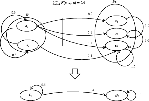
A stochastic bisimulation example. An MDP M of five states partitioned in two blocks (upper) that is reduced to an MDP M ′ with two abstract states (lower)
-
R(B 1,a)=−1, and
-
R(B 2,a)=0.

Based on these conditions, we can say that \(\mathcal {P} = \{B_{1}, B_{2}\}\) is a homogeneous partition that results in an MDP M ′ containing only two abstract states (Fig. 8 (lower)).
In order to find a stochastic bisimulation, we need to define an initial partition that can be a uniform partition with respect to the reward function. After that, we need to refine the partition blocks in order to make them stable, i.e., we refine them by splitting blocks that contain states that should not be together according to the transition function of these states. The process stops when all blocks are stable and the resulting partition is a stochastic bisimulation [6].
Definition 7.
(Reduced enumerative MDP) Given a partition \(\mathcal {P}\) that is a stochastic bisimulation, the reduced enumerative MDP [6] is defined as M ′=(S ′,A,P ′,R ′,γ), where S ′ is given by the blocks of \(\mathcal {P}\), i.e., \(B_{i} \in \mathcal {P}\) is an abstract state belonging to S ′; R ′(B i ,a)=R(s,a) for any s∈B i ; and \(P'(B_{w}|B_{j}, a) = \sum _{s' \in B_{w}} P(s'|s,a)\) for any s∈B j and for all B w ∈P, B j ∈P and a∈A.
Theorem 1.
Given a stochastic bisimulation \(\mathcal {P}\) for an MDP M and let M ′ be the reduced MDP obtained from \(\mathcal {P}\), then an optimal policy for M ′ is also optimal for M [ 6 ].
The advantage of solving M ′ is the possibility of doing less updates while looking for an optimal policy. For example, if s 1,s 5∈S and B i ={s 1,s 5}∈S ′, we can update only V(B i ) instead of V(s 1) and V(s 5), with the guarantee (Theorem 1) that in the optimal policy, π ∗(s 1)=π ∗(s 5)=π ∗(B 1).
Factored model reduction
Model reduction with factored splits (MRFS) is an algorithm to compute a homogeneous partition for factored MDPs [6]. MRFS can find a stochastic bisimulation using concepts of MDPs partitions combined with an operation called structure-based split (SS) [6], that refines a single block \(B_{j} \in \mathcal {P}\) with respect to a block \(B_{w} \in \mathcal {P}\) in order to generate sub-blocks stable with respect to \(B_{w} \in \mathcal {P}\). The SS operation receives a block \(B_{j} \in \mathcal {P}\), a block \(B_{w} \in \mathcal {P}\) and returns a partition \(\mathcal {P}'\) that is a refinement of \(\mathcal {P}\) in which B j is replaced by sub-blocks B j′={B1′,…,B l′} such that any sub-block in B j′ is stable with respect to B w (Definition 4). This is computed as follows [6]:
where \(\text {BS}\left (B_{j}, B_{w}, a\right) = B_{j} \cap \left (\bigcap _{X_{i} \in \text {vars}(B_{w})} \mathcal {P}_{X_{i}}^{a}\right)\) represents a block split considering one action and vars(B w ) is the set of state variables used to represent block B w [6]. When BS(B j ,B w ,a) is done, we have a partition of block B j that is stable with respect to B w considering only action a. To have B j′ stable with respect to B w , S S calls B S for each action a∈A and compute the intersection of the resultant partitions. The usage of vars(B w ) instead of all state variables in X is a way to efficiently compute the partitions, ignoring variables that will not affect the transition to block B w .
With SS, model reduction does not enumerate all states explicitly while refining blocks, since the splits are done using only the state variables in vars(B w ) to refine a block B j with respect to a block B w [6]. MRFS works as follows. The process starts with a uniform partition with respect to the reward function. After that, while the current partition \(\mathcal {P}\) contains a pair of blocks \(B_{j}, B_{w} \in \mathcal {P}\) such that B j is not stable with respect to B w , the process calls SS using B j and B w as parameters. In the refined partition, the sub-blocks of B j are stable with respect to B w [6].
MRFS can also be computed with ADDs [19] by generating a partition for each MDP function and refine them. To do this efficiently, we can ignore some of these partitions considering that in the factored MDP structure, we can have state variables that are irrelevant to model reduction [20]. Thus, model reduction can consider only the essential state variables, named X e . One way to compute X e is to add the state variables in \(\mathcal {P}^{A}_{R}\) to X e and, after that, recursively add the parents of those variables looking for the factored MDP DBNs [20]. Using the set X e , we can compute MRFS with ADDs as follows:
where \(\mathcal {P}^{A,R}_{\textit {DD}} = \bigotimes _{a \in A} \mathcal {P}^{a,R}_{\textit {DD}}\) and \(\mathcal {P}^{A,X_{e}}_{\textit {DD}} = \bigotimes _{a \in A} \left (\bigotimes _{X_{i} \in X_{e}} \mathcal {P}^{a,X_{i}}_{\textit {DD}}\right)\).
Methods
In the next sections we present the techniques that we use to improve model reduction performance.
Stochastic bisimulation over the reachable states
Suppose we have an MDP in which there is initial state information, that is, an MDP where we know a given initial state s 0∈S. MRFS can be improved if we use the reachable states information given s 0, specially in problems that have sparse transition matrixes, i.e., where the set of reachable states can be much smaller than the complete set of states.
Let \(\phantom {\dot {i}\!}S_{\text {reachable}|s_{0}}\) be the set of reachable states given s 0. If this set is computed before we look for a stochastic bisimulation, it is possible to get a reachability partition \(\mathcal {P}_{\textit {DD}}^{S|s_{0}} = \left \{\left (B_{\text {reachable}|s_{0}}, 1\right), \left (B_{\neg \text {reachable} |s_{0}}, 0\right)\right \}\phantom {\dot {i}\!}\), in which \(B_{\text {reachable}|s_{0}}\phantom {\dot {i}\!}\) represents the block of reachable states given \(s_{0}\left (S_{\text {reachable}|s_{0}}\right)\phantom {\dot {i}\!}\) and \(\phantom {\dot {i}\!}B_{\neg \text {reachable}|s_{0}}\) represents the block of unreachable states given \(\phantom {\dot {i}\!}s_{0}\left (S \backslash S_{\text {reachable}|s_{0}}\right)\).
Figure 9 summarizes three different kinds of partitions that could be done over a set of states S:
-
(a)
a partition in which the states in S are divided into |S| blocks, i.e., each block contains a single state;
Fig. 9 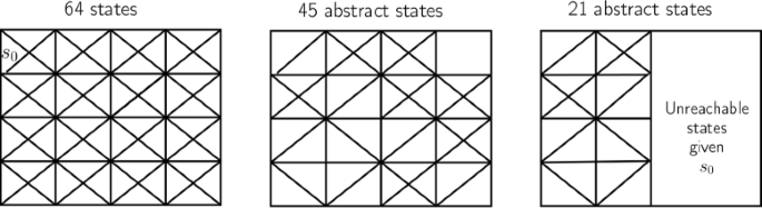
Different partitions of S. The first box represents a set of states. The second box is a partition of the first box, and the third box is also a partition of the first box but only over the reachable states given s 0
-
(b)
a partition over S in which each block can contain more than one state; and
-
(c)
a partition over S that has refinements only in the subset \(\phantom {\dot {i}\!}S_{\text {reachable}|s_{0}}\).

If we consider only partitions of item (c) to compute stochastic bisimulations, we can have the following advantages:
-
model reduction begins with smaller partitions, what makes computing more efficient; and
-
the reduced model can be smaller than (b).
To find \(\mathcal {P}_{\textit {DD}}^{S|s_{0}}\), it is necessary to visit all the reachable states given s 0. This procedure is done layer by layer, simulating each action of the MDP in each reachable state (similarly to a breadth-first search [21]). Reachable states can be efficiently computed representing the sets of states in each layer as BDDs [22] and using BDD operations such as union, intersection, and marginalization. Algorithm ?? shows how we compute the reachable states given an MDP M and a state s 0.

Reachability-based model reduction
Reachability-based MRFS (ReachMRFS) is an extended version of MRFS that computes stochastic bisimulations over \(S_{\text {reachable}|s_{0}}\phantom {\dot {i}\!}\). Hence, it is required to compute first the reachability partition, \(\mathcal {P}^{S|s_{0}}_{\textit {DD}}\) (Algorithm ??), and after that, we compute MRFS considering only the states in \(\phantom {\dot {i}\!}B_{\text {reachable}|s_{0}}\).

The algorithm ReachMRFS (Algorithm ??) works as follows. In the first external foreach, partitions \(\mathcal {P}^{a,R}_{\textit {DD}}\) are multiplied by the partition \(\mathcal {P}^{S|s_{0}}_{\textit {DD}}\), resulting in the partitions \(\mathcal {Q}^{a,R}_{\textit {DD}}\) (i.e., partitions based on the reward function for an action a over the reachability partition), where unreachable states are labeled with 0. As reachability partition has only two blocks, labeled with the values 0 and 1, when we compute the product of this partition with other MDP partitions, some leaves get the value 0 and others stay the same. In this way, many leaves can receive a value 0, which reduces the number of leaves and enables us to have a more compact representation. Furthermore, if we compute the refinements among partitions that were already simplified, the number of blocks in the refined partition is smaller than the number of partitions using all the possible states. The partitions \(\mathcal {Q}^{a,R}_{\textit {DD}}\) are used to compute a uniform partition with respect to the reward function (i.e., for all action a∈A) over S reachable, that we call \(\mathcal {P}^{a,R}_{\textit {DD}}\).
In the second external foreach, we compute a partition with stable blocks over the reachable states in the same way, by getting a simpler partition \(\mathcal {P}^{A,X}_{\textit {DD}}\). Finally, in the last two lines, we compute the stochastic bisimulation over reachable states and return it.
While MRFS computes the partition intersections as in Fig. 7, ReachMRFS use the reachability partition to simplify the computation. The advantages appear in two ways: (1) the program needs less space to store the ADDs in main memory and (2) the products among partitions can be done faster because many leaves are equal to 0, specially in problems with a sparse transition matrix. The benefits of ReachMRFS can be seen in Figs. 10 and 11 that shows the reduction in the size of the ADDs and hence, in the resulting partition when compared with the refinement in Fig. 7.

Partitions over the set of reachable states given s 0. The partitions \(\mathcal {P}_{1}\) and \(\mathcal {P}_{2}\) of Fig. 7 are multiplied by the resulting partition \(\mathcal {P}^{S|s_{0}}_{\textit {DD}}\), resulting in \(\mathcal {Q}_{1}\) and \(\mathcal {Q}_{2}\)

Reachability-based model reduction with partitions elimination
Another improvement to efficiently compute stochastic bisimulations is the elimination of repeated partitions computed by the algorithms MRFS and ReachMRFS. These algorithms use partitions based on reward and transition functions. In a general way, the maximum number of distinct MDP partitions used by these algorithms is at most |A|+(|A|×|X|). However, in practical situations, these partitions are not all distinct and if we compute the stochastic bisimulation using all these partitions, the process can be very slow.
Let \(\mathcal {P}\) and \(\mathcal {P}'\) be partitions of an MDP. We say that \(\mathcal {P} = \mathcal {P}'\) if \(|\mathcal {P}| = |\mathcal {P}'|\) and if for each \(B_{i} \in \mathcal {P}\) there is a block \(B_{j} \in \mathcal {P}'\) with the same DNF characterizing both of them. Based on this concept, a partition \(\mathcal {P}'\) obtained from a function f (reward or probabilistic transition) is repeated if the reduction algorithm found a partition \(\mathcal {P}\) (before \(\mathcal {P}'\)), obtained from a function g (reward or probabilistic transition), and we have \(\mathcal {P} = \mathcal {P}'\). Given a list of partitions L, we say the partitions are distinct among themselves if for each partition \(\mathcal {P}_{i} \in L\) obtained from an MDP function, L does not have \(\mathcal {P}_{j}\) obtained from another MDP function such that \(\mathcal {P}_{i} = \mathcal {P}_{j}\).
ReachMRFS-V2 (Algorithm ??) is a version of ReachMRFS that starts computing partition elimination and then computes the refinements among the partitions in L.

Results and discussion
In [23], we have shown that ReachMRFS-V2 can be much more efficient than MRFS, specially in sparse domains. At the same time, in dense domains, the overhead of reachability analysis does not affect the general performance of model reduction because we use efficient ADD operations to find the reachable states. In this work, we complete those results by including VI and TVI to solve the reduced MDP. Furthermore, we also solve the original MDP M using these three algorithms to identify the trade-offs of applying model reduction.
For all algorithms, we use γ=0.99 and ε=10−3. The methodology employed in experiments is to execute each algorithm until convergence enforcing a time and memory cutoff of 1 h and 3GB, respectively. The results are presented as the average and 95 % confidence interval over 30 executions for each pair of planner and problem. The experiments were conducted on a 2.4-GHz machine with 16 cores running a 64-bit version of Linux and our implementation was developed in Java using the official RDDL Simulator (RDDLSim) [24]. Our implementation is available in the following repository: http://github.com/felipemartinsss/repository/tree/master/AIPlannersForRDDLSim.
The benchmark problems were taken from the International Probabilistic Planning Competition (IPPC-2011), which were specified in RDDL (Relational Dynamic Influence Diagram Language) [24], a language to represent factored MDPs. In the IPPC-2011, there were eight domains with ten instances each and we selected the following domains for our experiments: Crossing Traffic, Elevators, Game of Life, Navigation and Skill Teaching.
Table 1 presents the comparison between ReachMRFS-V2 and MRFS using VI, TVI, and LRTDP as planners to solve the reduced MDP. As expected, the performance of the ReachMRFS-V2 dominates the performance of MRFS in all the problems, i.e., the slowest ReachMRFS-V2 planner (usually ReachMRFS-V2 + LRTDP) is faster than all planners that use MRFS planners. This is due the reachability analysis and partition elimination applied by ReachMRFS-V2.
Another interesting trend in Table 1 is that TVI (LRTDP) is the best (worst) planner for solving the reduced MDPs generated by both ReachMRFS-V2 and MRFS. The reason for this trend is the fact that all the states in the reduced MDPs are reachable from their initial states. Therefore, the sampling procedure of LRTDP is inefficient in comparison with the topological analysis applied by TVI since no state in the reduced MDPs can be ignored.
In Table 2, we compare ReachMRFS-V2 against no model reduction using VI, TVI, and LRTDP as planners.
For the Crossing Traffic domain, model reduction initially does not pay off and LRTDP has the best performance; however, as the size of the problem increases (problem #4), the reduced MDP is considerably smaller and ReachMRFS-V2 + TVI has the best overall performance.
In the Elevators domain, ReachMRFS-V2 + TVI is the overall best planner with ReachMRFS-V2 + VI being a closer runner-up. The reason for such performance is that the reachability analysis suffices to reduce the problem to a few thousand states. However, the reachable space contains only one strongly connected component, what is the worst case for TVI, therefore the overhead of the model reduction pays off when compared with TVI.
For the Game of Life domain, ReachMRFS-V2 + TVI dominates all the other planners and solve all the instances from three to ten times faster than the approaches without model reduction. This performance improvement is because the Game of Life problems are dense and all their states are reachable. Therefore, all the reduction obtained by ReachMRFS-V2 is due to the stochastic bisimulations.
For the Navigation domain, TVI has the best performance in almost all the instances because all the model reduction is due only to the reachability analysis; therefore, the stochastic bisimulations represent an expensive overhead.
For the Skill Teaching domain, LRTDP dominates all the other approaches because this domain is sparse and most of the model reduction is due to the reachability analysis. For instance, the problem number 4 has 224 possible states, only 1053 of them are reachable from s 0, and the reduced model has 702 states. Therefore, the stochastic bisimulation contributes with a negligible reduction in the model.
Conclusions
The experiment results show that model reduction always pays off when we have information about the initial state. For MDPs with dense transition function, the results show that stochastic bisimulation computation can explore the domain structure and, combined with the TVI planner to solve the reduced model, can have the best performance. For instance, the Game of Life domain problems with nine variables were solved in 2–3 min with ReachMRFS-V2 + TVI (while without the reduction, LRTDP takes 15–23 min). For sparse domains like Elevators and Crossing traffic, the results show that there is an overhead of the model reduction. However, for 8 out of 26 problems, this overhead pays off and ReachMRFS-V2-based planners are the best overall considered planners. It is a future research topic to find a general rule for deciding whenever ReachMRFS-V2 should be applied or not.
References
Puterman ML (1994) Markov decision processes: discrete stochastic dynamic programming. John Wiley & Sons, New York, NY, USA.
Hoey J, St-Aubin R, Hu A, Boutilier C (1999) SPUDD: Stochastic planning using decision diagrams In: Proceedings of the 15th Conference on Uncertainty in Artificial Intelligence, 279–288.. Morgan Kauffman, San Franciso, CA, USA.
Feng Z, Hansen EA, Zilberstein S (2003) Symbolic generalization for on-line planning In: Proceedings of the 19th Conference on Uncertainty in Artificial Intelligence, 109–116.. Morgan Kaufmann, San Francisco, CA, USA.
Barto AG, Bradtke SJ, Singh SP (1993) Learning to act using real-time dynamic programming. Artif Intell 72: 81–138.
Bonet B, Geffner H (2003) Labeled RTDP: improving the convergence of real-time dynamic programming In: Proceedings of 13th International Conference on Automated Planning and Scheduling, 12–21.. AAAI Press, ICAPS, Trento, Italy.
Givan R, Greig M, Dean T (2003) Equivalence notions and model minimization in Markov decision processes. Artif Intell 147: 163–223.
Bertsekas D, Tsitsiklis JN (1996) Neuro-dynamic programming. Athena Scientific, Cambridge, MA, USA.
Dean T, Kanazawa K (1990) A model for reasoning about persistence and causation. Comput Intell 5: 142–150.
Bahar RI, Frohm EA, Gaona CM, Hachtel GD, Macii E, Pardo A, Somenzi F (1993) Algebraic decision diagrams and their applications In: Proceedings of the 1993 IEEE/ACM International Conference on Computer-aided Design, 188–191.. IEEE Computer Society Press, Los Alamitos, CA, USA.
Bryant RE (1986) Graph-based algorithms for Boolean function manipulation. IEEE Trans Comput 35: 677–691.
Dai P, Goldsmith J (2007) Topological value iteration algorithm for Markov decision processes In: IJCAI’07 Proceedings of the 20th International Joint Conference on Artificial Intelligence, 1860–1865.. Morgan Kauffman, San Francisco, CA, USA.
Bertsekas DP (1995) Dynamic programming and optimal control. Vol. 1. Athena Scientific, Cambridge, MA, USA.
Li L, Walsh TJ, Littman ML (2006) Towards a unified theory of state abstraction for MDPs In: Proceedings of the 9th International Sysmposium on Artificial Intelligence and Mathematics, 531–539, Fort Lauderdale, Florida, USA.
Dean T, Givan R, Leach S (1997) Model reduction techniques for computing approximately optimal solutions for Markov decision processes In: Proceedings of the 13th Conference on Uncertainty in Artificial Intelligence, 124–131.. Morgan Kauffman, San Francisco, CA, USA.
Givan R, Leach S, Dean T (2000) Bounded-parameter Markov decision processes. Artif Intell 122: 71–109.
Ravindran B, Barto AG (2002) Model minimization in hierarchical reinforcement learning. Lecture Notes Comput Sci2371/2002: 196–211.
Ravindran B, Barto AG (2004) Approximate homomorphisms: a framework for non-exact minimization in Markov decision processes In: Proceedings of the 5th International Conference on Knowledge Based Computer Systems, Hyderabad, India.
Boutilier C, Dearden R, Goldszmidt M (1995) Exploiting structure in policy construction In: IJCAI-95, 1104–1111.. University of British Columbia Vancouver, BC, Canada, Canada.
Kim KE, Dean T (2002) Solving factored MDPs with large action space using algebraic decision diagrams In: Proceedings of the 7th Pacific Rim International Conference on Artificial Intelligence: Trends in Artificial Intelligence, 80–89.. Springer-Verlag, London, UK.
Guo W, Leong TY (2010) An analytic characterization of model minimization in factored Markov decision processes In: Proceedings of the 24th AAAI Conference on Artificial Intelligence, 1077–1082.. AAAI Press, Atlanta, Georgia.
Russel S, Norvig P (2003) Inteligência Artificial: Uma Abordagem Moderna. Segunda edn.. Campus/Elsevier, Rio de Janeiro.
Pednault EPD (October, 1994) ADL and the state-transition model of action. Journal of Logic and Computation, Volume 4, Number 5: 1077–1082.
dos Santos FM, de Barros LN, Holguin MG (2013) Stochastic bisimulation for mdps using reachability analysis In: 2013 Brazilian Conference on Intelligent Systems (BRACIS), 213–218, Fortaleza, Ceará, Brazil.
Sanner S (2010) Relational dynamic influence diagram language (RDDL): language description. http://users.cecs.anu.edu.au/~ssanner/IPPC_2011/RDDL.pdf.
Acknowledgements
The authors would like to thank:
∙ CAPES, for supporting FMS during the master degree research;
∙ FAPESP, for supporting FWT (process number 2013/11724-0);
∙ Mijail Gamarra Holguin, for helping with the implementation of the planners and the use of ADD library; and
∙ Karina Valdivia Delgado, for some ideas on factored representation and operations of MDPs.
Author information
Authors and Affiliations
Corresponding author
Additional information
Competing interests
The authors declare that they have no competing interests.
Authors’ contributions
This work is part of FMS Master thesis and LNB was his advisor. FMS carried out most of the investigation, implementation, experiments, and writing. LNB gave important ideas to the project and also contributed in the writing and revision of this manuscript. FWT gave important ideas about new techniques to solve MDPs and the implementation of the TVI algorithm and suggested a new series of experiments; he also gave an important contribution in writing and revising the paper. All authors read and approved the final manuscript.
Rights and permissions
Open Access This article is distributed under the terms of the Creative Commons Attribution 4.0 International License (https://creativecommons.org/licenses/by/4.0), which permits use, duplication, adaptation, distribution, and reproduction in any medium or format, as long as you give appropriate credit to the original author(s) and the source, provide a link to the Creative Commons license, and indicate if changes were made.
About this article

Cite this article
Santos, F.M., Barros, L.N. & Trevizan, F.W. Reachability-based model reduction for Markov decision process. J Braz Comput Soc 21, 5 (2015). https://doi.org/10.1186/s13173-015-0024-1
Received:
Accepted:
Published:
DOI: https://doi.org/10.1186/s13173-015-0024-1