Evaluation of linear relaxations in Ad Network optimization for online marketing

Abstract

Background

Ad Networks connect advertisers to websites that want to host advertisements. When users request websites, the Ad Network decides which ad to send so as to maximize the number of ads that are clicked by users. Due to the difficulty in solving such maximization problems, there are solutions in the literature that are based on linear programming (LP) relaxations.

Methods

We contribute with a formulation for the Ad Network optimization problem, where it is cast as a Markov decision process (MDP). We analyze theoretically the relative performance of MDP and LP solutions. We report on an empirical evaluation of solutions for LP relaxations, in which we analyze the effect of problem size in performance loss compared to the MDP solution.

Results

We show that in some configurations, the LP relaxations incur in approximately 58 % revenue loss when compared to MDP solutions. However, such relative loss decreases as problem size increases. We also propose new heuristics to improve the use of solutions achieved by LP relaxation.

Conclusions

We show that solutions obtained by LP relaxations are suitable for Ad Networks, as the performance loss introduced by such solutions are small in large problems observed in practice.

Background

In this paper, we analyze, theoretically and empirically, the performance of linear relaxations in Ad Network optimization — an essential component of online marketing. Online marketing is a form of marketing and advertising which uses the Internet to deliver promotional marketing messages to consumers. The economic importance of such a task is apparent. Indeed, online marketing revenue has grown quickly since mid-nineties, with a compound annual growth rate of 20 %. In the first semester of 2014, this market achieved a revenue of 23.1 billion dollars (USD) only in the USA, an astonishing growth of 15.1 % over the first semester of 2013 [1]. Revenue comes from search-related marketing (39 %), banner displaying (28 %), mobile advertising (23 %), and other activities (10 %).

Online advertising companies usually follow either an online or an offline model. Both models assume the existence of a broker that has contracts with websites. These websites have spaces where banners can be displayed. The online model works by real-time bidding; in this model, advertisers participate in auctions, normally a Vickrey auction [2], where the value to be paid by the auction’s winner is the second largest bid, competing for specific user profiles. In the offline model, advertisers establish contracts with a broker, from now on called the Ad Network. Advertisers create campaigns specifying a set of ads, a pricing model, a budget, a minimal number of impressions (an impression corresponds to the display of an ad to a user), and time restrictions (that is, how long the campaign will be available and its starting time). The Ad Network decides how to distribute these ads to the users, so as to maximize the Ad Network revenue, and respecting the conditions specified by the advertisers. This paper focuses only on the offline model.

There are several pricing models [3, 4]; however, the most used ones are cost per impression (CPI), cost per action (CPA), and the cost per click (CPC). In the CPI model, the advertiser pays only for a number of impressions of the campaign. In the CPA model, the advertiser pays by specific users’s actions, e.g., filling in a form or buying a product in the advertisers’ store. In the CPC model, the advertiser pays when the user actually clicks in the advertisement. In 2014, advertisers paid 34 % of online advertising transactions on a cost-per-impression basis, 65 % on customer performance (e.g., cost per click or cost per acquisition), and 1 % on hybrids of impression and performance methods. CPC’s market share has grown each year since its introduction, eclipsing CPI to dominate two-thirds of all online advertising pricing methods [5]. This paper focuses on the CPC pricing model.

The offline business model is, in essence, a sequential decision process: the Ad Network must decide which campaign to display to each user at a specific time, given campaign budgets, values that campaigns pay per click, time constraints of the campaigns, and the relationship between campaigns and user profiles. Ad Network decisions are evaluated based on some utility function; for example, expected revenue.

This sequential decision process can be modeled as a Markov decision process (MDP), as noticed by some authors [6].

The solution of this MDP yields the policy for the Ad Network, indicating the best decision for each possible combination of user profile, budget, and time constraints. However, this approach is computationally intractable even for small problems, as the state space grows exponentially with the number of state variables of the problem.

One way to avoid the curse of dimensionality in Ad Network optimization is to convert this decision process into a simpler, relaxed problem: Instead of deciding which campaign to allocate for each user profile at each time step, one then selects only the number of impressions of each campaign in a given interval of time. Some well-known formulations of this relaxed problem rely on linear programming (LP), which have produced good results [6, 7].

In this paper, we contribute with an explicit MDP formulation for the Ad Network problem and we compare it with the LP formulation for the relaxed problem. We have expanded the results of a previous paper [8] to present a detailed analysis of the behavior of the two formulations. In our analysis, we build scenarios that clearly show the loss of performance resulting from the use of the LP formulation when compared with the MDP formulation. However, we show that the LP results are indeed close to results obtained with MDP models when relatively large budgets are assigned to campaigns. Thus, the performance loss of the LP formulation drops when the campaign budgets reach realistic sizes. Finally, we also propose new heuristics to improve the use of solutions achieved by LP relaxation.

The remainder of this paper is organized as follows. “Problem definition” section formalizes the problem of Ad Network optimization. In “Ad Networks as a Markov decision process” section, we formulate the problem as an MDP, and in “A linear programming relaxation” section, we formulate the problem as a relaxed problem to be solved by LP. “Methods” section builds cases that are unfavorable for the LP formulation. “Results and discussion” section describes the experiments that allow us to highlight and discuss the differences between the solutions for the MDP and LP models. “Conclusions” section concludes the paper.

Problem definition

Ad Networks promote the distribution of ads to websites [9]. Advertisers create ads, grouped in campaigns, and publishers are websites that own spaces for the display of ads. Campaigns are designed by advertisers.

The campaigns processed by the Ad Network are described by the campaign set $\mathcal {C}$. A campaign $k \in \mathcal {C}$ is defined by a tuple <B _k ,S _k ,L _k ,c c _k >, where B _k is the budget of campaign k in number of clicks, S _k is the starting time of the campaign, L _k is the lifetime of the campaign, and c c _k is the monetary value that the campaign pays per click. Campaigns can be active or inactive, and only active campaigns can be chosen by the Ad Network. A campaign is active at a specific time t if S _k ≤t<S _k +L _k and the remaining budget is larger than zero.

The advertisers contract the service of an Ad Network to display ads of campaigns in websites, providing to the Ad Network a set of campaigns. It is also assumed that these contracts occur previously to the beginning of the distribution of ads. Figure 1 depicts the flow of ad distribution in online marketing.

Fig. 1

Dynamics of the ad distribution process

Every time a user requests a page in a website (step 1 in Fig. 1), the website requests an ad to be displayed (step 2). Users are characterized by their profiles, and these are known by the Ad Network. The Ad Network decides which campaign to allocate to the received request, and an ad of the selected campaign is sent to the website (step 3). Then, an impression is made, i.e., the ad is displayed as a banner to the user (step 4), who may or may not click on the ad (step 5).

This sequential process can be formalized as follows. At each time t, there is a probability that a request is received by the Ad Network; that is, a probability of a user requesting a page in a site in the Ad Network’s inventory. We assume that the requests follow a Bernoulli distribution with a success probability P _req. This modeling decision is justified as the Bernoulli distribution is well suited to encode the arrival of random requests from a large unknown population [10].

Users are classified into different profiles, and the set of possible user profiles is denoted by $\mathcal {G}$. A probability distribution $P_{\mathcal {G}}: \mathcal {G} \rightarrow [0,1]$ yields the probability that a user belongs to a user profile i.

Once the campaign k is selected, one of its ads is displayed to the user with profile i in a banner inside a page in a website.

The user may or may not click on this ad with probability CTR(i,k), where CTR stands for click-through rate. That is, CTR $: \mathcal {G} \times \mathcal {C} \rightarrow [0,1]$ is the probability of a click given a user profile and a campaign. In real problems, CTR values are typically on the order of 10⁻⁴ [6]. One click generates a revenue equal to c c _k ; a percentage of this amount goes to the website and the remaining revenue stays with the Ad Network.

The goal of the Ad Network is to choose which campaign to allocate to each request, while maximizing a utility function. We assume the Ad Network to be interested in maximizing expected revenue.

Ad Networks as a Markov decision process

We now formulate the Ad Network problem as an MDP. The formulation is based on our previous work on Ad Network optimization [8, 11].

A finite discrete-time fully observable MDP is a tuple $\langle \mathcal {S},\mathcal {A}, \mathcal {D}, \mathcal {T}, \mathcal {R}\rangle$ [12], where:

• $\mathcal {S}$ is a finite set of fully observable states of the process;

• $\mathcal {A}$ is a finite set of all the possible actions to be executed at each state; $\mathcal {A}(s,t)$ denotes the set of valid actions at instant t when the system is in state $s \in \mathcal {S}$;

• $\mathcal {D}$ is a finite sequence of natural numbers that correspond to decision epochs, in which the actions should be chosen and performed;

• $\mathcal {T}:\mathcal {S}\times \mathcal {A}\times \mathcal {S}\times \mathcal {D}\rightarrow [0,1]$ is a transition function that specifies the probability $\mathcal {T}(s,a,s',t)$ that the system moves to state s ^′ when action a is executed in state s at time t;

• is a reward function that produces a finite numerical value $r = \mathcal {R}(s,a,s',t)$ when the system goes from state s to state s ^′ as a result of applying an action a at time t.

An MDP agent is continuously in a cycle of perception and action (Fig. 2): at each time t the agent observes the state $s \in \mathcal {S}$ and decides which action $a \in \mathcal {A}(s,t)$ to perform; the execution of this action causes the transition to a new state s ^′ according to the transition probability function $\mathcal {T}$ and the agent receives a reward r. This cycle is repeated until a stopping criterion is met; for example, until there are no more valid decision epochs.

Fig. 2

Perception and action cycle — The agent observes the state, applies an action, receives a reward, and observes the new state

It is important to notice that this system is not deterministic. Given a transition function $\mathcal {T}$, when the same action is performed in the same state and at the same instant of time, the system may move to different states.

To solve an MDP is to find a policy that maximizes the accumulated reward sequence. A non-stationary deterministic policy $\pi :\mathcal {S}\times \mathcal {D} \rightarrow \mathcal {A}$ specifies which action $a \in \mathcal {A}$ will be executed at each state $s \in \mathcal {S}$ and at time $t \in \mathcal {D}$, $\mathcal {D} = \{0,1,\ldots,\tau -1\}$.

The expected total reward of a policy π starting at time t at state $s\in \mathcal {S}$ is defined as:

$$ V^{\pi}(s,t) = \mathrm{E}\left.\left[\sum_{i=t}^{\tau-1}\mathcal{R}(s_{i},\pi(s_{i},t), s_{i+1},t)\right|s_{t}=s,\pi\right]. $$

((1))

The value function V ^∗ of an optimal policy can be defined recursively for any state $s\in \mathcal {S}$ and time t<τ by:

$${} {\fontsize{8.8pt}{9.6pt}\selectfont{\begin{aligned} V^{*}(s,t) = \max_{a\in\mathcal{A}(s,t)}\left\{ \sum_{s' \in \mathcal{S}} \mathcal{R}(s,a,s',t) + \mathcal{T}(s,a,s',t)V^{*}(s',t+1)\right\}\!, \end{aligned}}} $$

((2))

where $\mathcal {A}(s,t)$ is the subset of $\mathcal {A}$ which contains the possible actions to be applied in state s at time t, and V ^∗(s,τ)=0 for any state $s\in \mathcal {S}$ [13].

Given the optimal value function V ^∗(·), an optimal policy can be chosen for any state $s\in \mathcal {S}$ and time t<τ by:

$${} {\fontsize{8.6pt}{9.6pt}\selectfont{\begin{aligned} \pi^{*}(s,t) = \arg\max_{a\in\mathcal{A}(s,t)}\left\{\!\sum_{s' \in \mathcal{S}} \!\mathcal{R}(s,a,s',t)\!+\mathcal{T}(s,a,s',t)V^{*}(s',t+1)\!\right\}\!. \end{aligned}}} $$

The intuition behind the expressions above is exploited by the value iteration algorithm [14], described in Algorithm 1.

Once the optimal policy π ^∗ is available, just apply it at every decision epoch: the agent observes the state s and instant of time t and applies the action defined by the optimal policy, a=π ^∗(s,t).

For the problem of Ad Networks, the network observes its current state, given by the configuration of the campaigns and the user profile, and then the optimal policy defines the campaign to be displayed on the website.

We now contribute with a model for the Ad Network problem as an MDP by specifying its states, actions, transitions, and rewards.

States

The state is modeled as:

$$s = \left[ B_{1}, B_{2}, \dots, B_{k}, G \right], $$

where B _i is the remaining budget of campaign i and $G \in \mathcal {G} \cup \{0\}$ is the user profile that is generating a request. When the variable G is equal to 0, there is no request to attend to. For example, consider 5 campaigns and 3 user profiles, a state could be:

$$\underbrace{[\overbrace{10, 3, 4, 2, 3}^{\text{Campaign information}}, \overbrace{3}^{\text{Request information}}]}_{\text{State}}. $$

Here, campaign 1 can afford 10 clicks, campaign 2 can afford 3 clicks, and so on. The request information contains the information of which user profile has generated a request; in this example, user profile i=3 has generated the request. From this state, possible next states are: [9,3,4,2,3,G], [10,2,4,2,3,G], [10,3,3,2,3,G], [10,3,4,1,3,G], [10,3,4,2,2,G], and [10,3,4,2,3,G], where G can be any user profile in $\mathcal {G}$ or even 0, if there are no requests in the next time step.

Actions

An action allocates an ad from a campaign in the set $\mathcal {C}$ to a request from a user profile in set $\mathcal {G}$. Given our problem definition, the set of actions can be defined by $\mathcal {A}=\{0,1,\ldots,|\mathcal {C}|\}$ and an action is simply an integer k. If k>0, then k is the campaign index, $k \in \{1,2, \dots, |\mathcal {C}|\}$. If k=0, then the Ad Network does not allocate any campaign to the user request.

Recall that campaigns can be active or inactive, hence at any time t a subset of actions $\mathcal {A}(s,t)$ is available, consisting of action 0 plus all k>0 such that S _k ≤t<S _k +L _k and such that B _k >0.

Transitions

For all actions a and all states s and s ^′, the function $\mathcal {T}$ must satisfy the following requirements: $0 \leq \mathcal {T}(s,a,s',t) \leq 1$, and $\sum _{s' \in \mathcal {S}}\mathcal {T}(s,a,s',t) = 1$.

The variable G in the state does not depend on the previous state. The component of the state B k′ depends only on the previous B _k and on the occurrence of click events. Given s=[B ₁,B ₂,…,B _j ,G] and s ^′=[B1′,B2′,…,B j′,G ^′], the transition function $\mathcal {T}$ is:

$$ \mathcal{T}(s,a,s',t) = P_{t}(G') \times \prod_{k\in\mathcal{C}}P(B'_{k}|B_{k},a,G), $$

((3))

where P(B k′|B _k ,a,G) is equal to:

$${} {\fontsize{8.6pt}{9.6pt}\selectfont{\begin{aligned} \left\{ \begin{array}{llll} 1 & \text{if}~ B_{k}'=B_{k}~\text{and}~ (a \neq k ~\text{or}~ G=0~\text{or}~B_{k}=0), \\\\ \text{CTR}(G,k) & \text{if}~ B_{k}'\,=\,B_{k}-1 ~\text{and}~ (a \,=\, k ~\text{and}~ G\!>\!0 ~\text{and}~ B_{k}\!>\!0), \\\\ 1-\text{CTR}(G,k) & \text{if}~B_{k}'=B_{k} ~\text{and}~ (a = k ~\text{and}~ G>0 ~\text{and}~ B_{k}>0), \\\\ 0 &\text{otherwise,} \end{array}\right. \end{aligned}}} $$

((4))

and

$$ P_{t}(G') =\left\{ \begin{array}{ll} (1-P_{\text{req}}) & \text{if}~G' = 0, \\ P_{\text{req}}\times P_{\mathcal{G}}(G) & \text{if}~ G'\in\mathcal{G},\\ \end{array}\right. $$

((5))

where P _req is the probability that a request is received by the Ad Network, and $P_{\mathcal {G}}$ is the probability of a user being of a given user profile. Note that the transition function $\mathcal {T}$ is time-invariant.

As an example, consider the problem in which P _req=0.9, $\mathcal {G}=\{1,2\}$, B ₁=B ₂≥2, $P_{\mathcal {G}}(G) = \frac {1}{|\mathcal {G}|}=0.5$, and CTR(i,k)=i×k×10⁻⁴. From the state s=[B ₁,B ₂,1], there is the possibility of 12 future states. Figure 3 illustrates some examples; therein, if a=1 then

• $P1 = P_{\text {req}} \times P_{\mathcal {G}} \times (1 - \text {CTR}(1,1)) \times 1 = 0.9 \times 0.5$ ×(1−1×1×10⁻⁴)×1,

  Fig. 3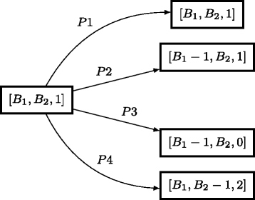

  

  Some examples of next states when action 1 is performed in state s=[B ₁,B ₂,1]

• $P2 = P_{\text {req}} \times P_{\mathcal {G}} \times \text {CTR}(1,1) \times 1 =0.9\times 0.5$ ×(1×1×10⁻⁴)×1,

• P3=(1−P _req)×CTR(1,1)×1=(1−0.9) ×(1×1×10⁻⁴)×1,

• $P4 = P_{\text {req}} \times P_{\mathcal {G}} \times (1 - \text {CTR}(1,1)) \times 0 = 0.9\times 0.5$ ×(1−1×1×10⁻⁴)×0.

Rewards

In our model, we assume that the reward does not vary over time, and that it is independent of the next state. Thus, the reward function is . In our problem, we have:

$${} {\fontsize{8.8pt}{9.6pt}\selectfont{\begin{aligned} \mathcal{R}(s,a) =\left\{ \begin{array}{ll} cc_{k}\times \text{CTR}(G,k) & \text{if \(a>0, a=k\), \(G>0\) and \(B_{k}>0\),} \\ 0 & \text{otherwise,}\\ \end{array}\right. \end{aligned}}} $$

((6))

where c c _k and CTR(G,k) were defined in “Problem definition” section and specify respectively the CPC for campaign k and the CTR for campaign k and user profile G. The intuition behind the reward function is that it represents the local revenue after choosing to display an ad from campaign k.

A linear programming relaxation

Here, we formulate the Ad Network problem as an LP relaxation. LP focuses on maximization or minimization of a linear function over a polyhedron [15]. In canonical form, we must find

$$\begin{array}{ll} \max & \quad c^{T}x \\ s.t. & \quad Ax \leq b, \quad x \geq 0, \end{array} $$

where c and b are vectors, A is a matrix, and x is a vector of variables. There are several algorithms to solve an LP problem, even strongly polynomial time algorithms [16]. The simplex method is the most commonly used [17]; despite its worst-case exponential time, this method is in average very efficient [18].

In the Ad Network relaxation, we are interested in discovering the number of ad displays to be allocated for each campaign in a given interval of time. The description that follows is based on previous efforts [6, 7] with minor modifications¹.

Let $\mathcal {I}$ be a sorted list obtained by sorting the set defined by {S _k }∪{S _k +L _k }; that is, the ordered list of starting and ending times of all campaigns, and let $\mathcal {J}_{j}$ be the (right-open) set of intervals defined by the campaign time constraints. Define $\mathbb {T}_{j}$ to be the length of the interval j.

For example, in Fig. 4, we have three campaigns, with their starting times and ending times, defining five intervals. Consider that E _k =S _k +L _k . In this example, we have that: $\mathcal {I} = \{S_{2},S_{3},S_{1},S_{3}+L_{3},S_{2}+L_{2},S_{1}+L_{1}\}$, then $\mathcal {J}_{1}= [S_{2},S_{3}[$, $\mathcal {J}_{2}= [S_{3},S_{1}[$, $\mathcal {J}_{3}= [S_{1},E_{3}[$, $\mathcal {J}_{4}= [E_{3},E_{2}$ $[,\mathcal {J}_{5}= [E_{2},E_{1}[$, and $\mathbb {T}_{1}=S_{3}-S_{2}$, $\mathbb {T}_{2}=S_{1}-S_{3}$, $\mathbb {T}_{3}=E_{3}-S_{1}$, $\mathbb {T}_{4}=E_{2}-E_{3}$, $\mathbb {T}_{5}=E_{1}-E_{2}$.

Fig. 4

Interval starting and ending points

We can state the LP approach to Ad Network optimization problem as follows:

$$\begin{array}{@{}rcl@{}} \max \quad \sum_{j \in \mathcal{J}} \sum_{i \in \mathcal{G}} \sum_{k \in \mathcal{C}} cc_{k} \times \text{CTR}(i,k) \times x_{j,i,k} \end{array} $$

((7))

$$\begin{array}{@{}rcl@{}} &s.t.& \sum_{k \in \mathcal{C}_{j}} x_{j,i,k} \leq P_{\text{req}} \times P_{\mathcal{G}}(i) \times \mathbb{T}_{j}, \forall i \in \mathcal{G}, \forall j \in \mathcal{J} \end{array} $$

((8))

$$\begin{array}{@{}rcl@{}} && \sum_{i \in \mathcal{G}} \sum_{j \in \mathcal{J}} \text{CTR}(i,k) \times x_{j,i,k} \leq B_{k}, \forall k \in {\mathcal{C}} \end{array} $$

((9))

$$\begin{array}{@{}rcl@{}} && x_{j,i,k} \geq 0, \forall j \in \mathcal{J}, \forall k \in \mathcal{C}, \forall i \in \mathcal{G} \end{array} $$

((10))

Variable x _j,i,k indicates how many ads from campaign k should be displayed to users with user profile i at the interval j. The objective function maximizes the total expected revenue of the Ad Network. The first set of constraints ensures that the solution does not exceed the expected number of requests for each user profile i in interval j. The second set of constraints ensures that the expected number of clicks for each campaign does not exceed its budget. The last set of constraints ensures that the solution is positive and therefore feasible for real problems. Without the last set of constraints, it would be possible to create requests for allocations with negative values of x _j,i,k . Clearly, x _j,i,k should be an integer because it is not possible to allocate a fraction of an ad, but we ignore (relax) this for now. Table 1 summarizes the list of symbols that we use.

Table 1 List of symbols

Policies for setting the ad to be displayed from the LP solution

Note that the LP solution indicates how many ads from campaigns should be shown to each user profile at each interval, but it does not provide any clue on how to apply this solution. Girgin et al. [6] proposed two ways to use the solution of this LP problem:

• 1. The highest LP policy (HLP), π _LP(i,j), selects the campaign in $\mathbb {T}_{j}$, where

  $$\pi_{\text{LP}}(i,j) = \arg\max_{k}\; x_{j,i,k}/\sum_{k} x_{j,i,k}. $$

• 2. The stochastic LP policy (SLP) selects stochastically with respect to “probabilities”

  $$x_{j,i,k}/\sum_{k} x_{j,i,k}. $$

Complexity of the MDP and the LP formulations

Here, we compare the complexity of the MDP formulation and the LP relaxation.

In the LP formulation, if the constraint (10), x _j,i,k ≥0, is not considered, the number of constraints is of order $O(|\mathcal {J}| \times | \mathcal {G} | + | \mathcal {C} |)$. But by definition $1 \leq |\mathcal {J}| \leq 2 \times |\mathcal {C}|$. Then, the number of constraints is of order $O(|\mathcal {G}||\mathcal {C}|)$, while the number of variables is of order $O(|\mathcal {G}||\mathcal {C}|^{2})$ for the same reason.

On the other hand, in the MDP formulation, the size of the policy to be found is equal to $|\mathcal {S}| \times |\{0,1,2,\dots,\tau -1\}|$, and $|\mathcal {S}| = (|\mathcal {G}| +1) \times \prod _{k \in \mathcal {C}} (B_{k} +1)$. If we consider $B_{\text {min}} = \min _{k \in \mathcal {C}}\{B_{k}\}$, it follows that $|\mathcal {S}| \geq (|\mathcal {G}| +1) \times (B_{\text {min}}+1)^{|\mathcal {C}|}$. This makes the MDP solution intractable even for small problems because of its memory requirements. In real settings, there are hundreds of campaigns with budgets of thousands of clicks.

Thus, despite the fact that the MDP formulation is a more faithful scheme, the LP formulation is computationally much more attractive. However, the LP formulation only indicates how many campaigns should be allocated in a given time interval, leaving the actual action to auxiliary schemes (for instance, HLP and SLP).

Methods

As discussed in the previous section, the relaxed LP formulation requires less computational effort than the MDP formulation. The LP relaxation approximates discrete actions by continuous ones, and its computational cost does not depend on budgets and time horizons. Because the relaxation ignores features of the original problem, it does not guarantee optimality.

In this section, we investigate the performance of LP relaxations by constructing simple scenarios where MDP optimal policies are clearly superior. We look at scenarios that are quite unfavorable for the LP formulation in order to understand how much can be lost with its use. At the end of this section, we propose a heuristic that can improve the use of solutions found with the LP formulation, based on insights obtained in our analysis.

A two-campaign one-profile scenario

Suppose we have just two campaigns and one user profile; to simplify the analysis, suppose both campaigns last for very long time, i.e., long enough to spend the budget for each campaign. We use η _k for the average cost per impression of campaign k; that is, η _k =c c _k ×CTR(1,k). We name ctr₁=CTR(1,1) and ctr₂=CTR(1,2). Without loss of generality, we take η ₁>η ₂, that is, campaign 1 pays more than campaign 2 and we say that campaign 1 is better than campaign 2.

When both campaigns have no time overlap, both MDP and LP solutions consist of showing the active campaign ads in the time slot in which the respective campaign is active. In this case, there is no difference between the performance of the two solutions.

Now suppose that the two campaigns have distinct starting times. The case where campaign 1 starts first is clearly less favorable to the LP formulation than the case where campaign 2 starts first. To conclude this, first consider the latter case; that is, the worst campaign starts first. In this case, we have $\mathbb {T}_{1}=S_{1}-S_{2}$, E ₁=E ₂=E→∞, and $\mathbb {T}_{2}=E-S_{1}$. The two solutions (for the MDP and the LP formulations) show the ads of the campaign 2 in $\mathbb {T}_{1}$. Since campaign 2 is the worst campaign, campaign 1 is always preferred to be showed unless all the budget B ₁ is spent. Notice that budget B ₂ is not spent unless there is enough time in intervals where only campaign 2 is active or budget B ₁ is spent. Finally, intervals where only campaign 2 is active do not influence intervals where both campaigns are active. Then, in a relative performance comparison, intervals where only the worst campaign 2 is active favor the worse method, LP formulation.

Now consider the former case; that is, the best campaign starts first. This is a case where the optimal solution of the MDP formulation can be “smarter” than the solution of the LP formulation. In this case, we have $\mathbb {T}_{1}=S_{2}-S_{1}$, E ₁=E ₂=E→∞, and $\mathbb {T}_{2}=E-S_{2}$. The expected number of clicks in $\mathbb {T}_{1}$ is $\beta = \mathbb {T}_{1} \times P_{\text {req}} \times \text {ctr}_{1}$. If β<B ₁, then the LP solution considers that budget B ₁ is not spent in interval $\mathbb {T}_{1}$ and assigns impressions to both campaigns during $\mathbb {T}_{2}$. If instead β>B ₁, then the LP solution considers that after $\mathbb {T}_{1}$ budget B ₁ was spent, and in interval $\mathbb {T}_{2}$, the LP relaxation only assigns impressions to campaign 2; this can be sub-optimal with respect to the MDP solution in case actual operation does not exhaust B ₁ during $\mathbb {T}_{1}$. And the worst case from the point of view of the LP relaxation is β=B ₁. For in this case, in interval $\mathbb {T}_{2}$, the LP relaxation only assigns impressions to campaign 2, while the MDP solution can flexibly use impressions from campaign 1 during $\mathbb {T}_{2}$ to exhaust B ₁.

We analyze this latter case in greater depth, which is depicted in Fig. 5.

Fig. 5

Two campaigns, best campaign starts first

In this case, the solution to the LP relaxation selects campaign 2 during $\mathbb {T}_{2}$, regardless of η ₂; it is clear that we subject the relaxation to larger loss (relative to optimal behavior) if we drive down η ₂. Consider then that η ₂=0; this may be an unrealistic scenario, but it does cause the solution to the LP relaxation to behave sub-optimally. Note that in such a case, we know that the MDP solution will reap the benefits of complete look-ahead, thus producing a value function V ^∗=B ₁. On the other hand, the Ad Network gets the following expected revenue when it applies the solution of the LP relaxation:

$${} R= cc_{1}\displaystyle \sum_{b=1}^{\mathbb{T}_{1}} \min\{b,B_{1}\}\binom{\mathbb{T}_{1}}{b}(P_{\text{req}}\ \text{ctr}_{1})^{b}(1-P_{\text{req}}\ \text{ctr}_{1})^{\mathbb{T}_{1}-b}. $$

Consequently, the relative performance is B ₁/R; that is,

$${} \frac{B_{1}}{cc_{1}\displaystyle \sum_{b=1}^{\mathbb{T}_{1}} \min\{b,B_{1}\}\binom{\mathbb{T}_{1}}{b}(P_{\text{req}}\ \text{ctr}_{1})^{b}(1-P_{\text{req}}\ \text{ctr}_{1})^{\mathbb{T}_{1}-b}}. $$

((11))

We can obtain a closed-form solution in some special cases. In particular, we consider one case that can be motivated as follows. In Expression (11), the numerator is the expected value of a binomial distribution with parameters $(\mathbb {T}_{1},P_{\text {req}}\text {ctr}_{1})$, while the denominator is the expected value of the same binomial distribution now truncated at B ₁. The difference between these distributions increases as the variance of the binomial distribution increases. To increase the distance between these quantities, we must choose B ₁ and ctr₁ so as to maximize the variance of the binomial relative to its mean. We can do so by reducing B ₁ and ctr₁; at a fixed B ₁, we reduce ctr₁ by increasing $\mathbb {T}_{1}$ as we have the constraint $B_{1} = \mathbb {T}_{1}P_{\text {req}}\ \text {ctr}_{1}$.

So, take B ₁=1. Then, we have the relative performance:

$$\frac{B_{1}}{R} = \frac{1}{1 - (1-P_{\text{req}}\ \text{ctr}_{1})^{\mathbb{T}_{1}}}; $$

in the limit, as $\mathbb {T}_{1}$ grows, we have:

$$\frac{B_{1}}{R} = {\lim}_{\mathbb{T}_{1} \rightarrow \infty} \frac{1}{1 - (1-P_{\text{req}}\ \text{ctr}_{1})^{\mathbb{T}_{1}}}. $$

Now recall that $P_{\text {req}}\ \text {ctr}_{1}=B_{1}/\mathbb {T}_{1}=1/\mathbb {T}_{1}$ under our assumptions, so we have the limiting relative performance

$$\frac{B_{1}}{R} = {\lim}_{\mathbb{T}_{1} \rightarrow \infty} \frac{1}{1 - (1-1/\mathbb{T}_{1})^{\mathbb{T}_{1}}} = \frac{e}{e-1} \approx 1.582. $$

This result suggests that, at least under some rather extreme circumstance, the LP relaxation can lead to a significantly poorer solution than the optimal one. What we will see experimentally later is that in realistic scenarios this potentially big difference is not at all realized; in fact, our ultimate conclusion is that the LP relaxation performs quite well in practical situations. Before we do so, we propose in the next section methods that can further improve the existing LP relaxations.

Improving solutions to the LP formulation

Girgin et al. [6] suggest that one should artificially increase the budget of high average-cost-per-impression campaigns, although it is difficult to determine how much should be increased to improve performance. More precisely, in the LP relaxation, one should take $B_{1}^{'} = \gamma B_{1}$ with γ>1.

In this section, we propose a value of γ, by comparing two possible scenarios, one which is unfavorable to the LP relaxation, and the other which is favorable to the LP relaxation.

Our first scenario is this. Given a factor γ, consider the Ad Network with two campaigns where η ₁>η ₂, S ₁<S ₂, $S_{2} - S_{1} = \mathbb {T}_{1} \to \infty$, $E_{1} = E_{2} = \mathbb {T}_{2} \to \infty$, B ₁=1, $\text {ctr}_{1} = \frac {\gamma B_{1}}{\mathbb {T}_{1}P_{\text {req}}}$, and ctr₂=0. Following the same reasoning as in the previous section, we find that the relative performance of the solutions for the MDP and the LP formulations is:

$$ \frac{V^{\pi_{\text{MDP}}}}{V^{\pi_{\text{LP}}}} = \left(\frac{e^{\gamma}}{e^{\gamma}-1}\right). $$

Now, consider a second scenario. Given a factor γ, consider the Ad Network with two campaigns where η ₁>η ₂ and η ₂→η ₁, S ₁=S ₂, L ₁=2 and L ₂=1, B ₁=1, B ₂=2, $\text {ctr}_{1} = \frac {\gamma B_{1}}{L_{1}P_{\text {req}}}$, ctr₂→ctr₁, and c c ₁=c c ₂.

Note that the solution to the LP relaxation uses campaign 1 in both intervals; and the solution to the LP relaxation does not use campaign 2. Then, the expected revenue of the LP relaxation is:

$$\begin{aligned} &cc_{1}\sum_{b=1}^{L_{1}} \min\{b,B_{1}\}\texttt{binopdf}\left(b;L_{1},\frac{\gamma}{2}\right)\\ &\quad= cc_{1}\left(1-\left(1 - \frac{\gamma}{2}\right)^{2}\right)=cc_{1}\left(\gamma-\frac{\gamma^{2}}{4}\right), \end{aligned} $$

where binopdf(s;n,p) is the binomial distribution of s with n trials and probability p. By taking η ₂→η ₁, the solution to the MDP formulation may choose any campaign, with value:

$$\begin{aligned} &cc_{1}\displaystyle\sum_{b=1}^{L_{1}} b \ \texttt{binopdf}\left(b;L_{1},\frac{\gamma}{2}\right) = cc_{1}\left(2\frac{\gamma}{2}\left(1-\frac{\gamma}{2}\right)\right)\\ &\quad+ 2cc_{1}\frac{\gamma^{2}}{4}=cc_{1}\gamma. \end{aligned} $$

Hence, the relative performance of an optimal solution (MDP) against the solution for the LP relaxation is:

$$\frac{4\gamma}{4\gamma-\gamma^{2}}. $$

Figure 6 shows how performances in these two scenarios vary with γ. Taking the best value in both scenarios, we have γ=1.202 as the best choice and relative performance 1.430.

Fig. 6

Relative performance of the solution of the MDP formulation against the solution of the LP relaxation with $B^{'}_{1}=\gamma B_{1}$

Results and discussion

To compare the results given by the MDP and the LP formulations, we conducted experiments with the two scenarios described in “Improving solutions to the LP formulation” section. We explore different settings for parameters B ₁, B ₂, $\mathbb {T}_{1}$, $\mathbb {T}_{2}$, and ctr₂, with c c ₁=c c ₂. In the first scenario described, we set:

$$\text{ctr}_{1} = \frac{B_{1}}{ P_{\text{req}}\mathbb{T}_{1}}, $$

while in the second scenario, we set:

$$\text{ctr}_{1} = \frac{B_{1}}{ P_{\text{req}}(\mathbb{T}_{1}+\mathbb{T}_{2})}. $$

First scenario

Consider the first scenario. We conducted experiments to study how the ratio $V^{\pi _{\text {MDP}}}/V^{\pi _{\text {LP}}}\phantom {\dot {i}\!}$ evolves when the budget increases in four different settings. In all such settings, we set $\mathbb {T}_{1}=50,000\phantom {\dot {i}\!}$. The first setting focuses on the LP formulation unfavorable scenario (shown in Fig. 5), named here as “the worst case scenario,” where B ₁=1, $\mathbb {T}_{2}\rightarrow \infty$, ctr₂=0. The second setting changes the size of the second interval by using $\mathbb {T}_{2}=50,000$. In this case, the Ad Network does not have infinite time to consume the budget of campaign 1. The third setting changes the budget and ctr₂ by using B ₂=B ₁, ctr₂=0.1×ctr₁. In this case, campaign 1 is much more attractive than campaign 2, but the LP formulation can now get some revenue during the second interval. The fourth setting changes ctr₂ to be closer to ctr₁, by setting ctr₂=0.5×ctr₁. Note that from the first to the fourth settings, the value of the solution of the LP formulation gets closer and closer to the value of the MDP formulation.

The idea in this experiment is to verify the relative performance of the two formulations. We go from a clearly unfavorable scenario for the LP formulation (the worst scenario) to a more realistic scenario by gradually increasing the budget. The experiment is conducted for this scenario in the four described settings.

Figure 7 shows the relative performance of solutions in these four settings for the first scenario. We can clearly see that the difference between the optimal solution (MDP) and the approximated solution (LP) is a decreasing function of the budget size. For clarity, Fig. 7 stops at B _k =50 and Fig. 8 considers values of B _k from 150 up to 200. With a budget of 20 clicks, the relative performance in all settings is less than 10 %; with a budget of 50 clicks, all settings have a relative performance smaller than 6 %. In Fig. 8, we can see that the setting with ctr₂=0 leads to the same result of the unfavorable scenario, and the relative performance still decreases. For B _k =200, we obtain a difference of about 2.90 % in the worst scenario and about 0.96 % in a slightly better setting.

Fig. 7

Relative performance of MDP against LP formulations for $\mathbb {T}_{2}=50,000$ and $\mathbb {T}_{2}\rightarrow \infty$ (the worst scenario), and budgets from 1 to 50

Fig. 8

Relative performance of MDP against LP formulations for $\mathbb {T}_{2}=50,000$ and $\mathbb {T}_{2}\rightarrow \infty$ (the worst scenario), and budgets from 150 to 200

Thus, we observe that the performance loss by the LP formulation decreases significantly as we explore more realistic situations.

Second scenario

Consider now the second scenario. Again, we build four settings for this scenario. The first setting we consider is the worst case one, $B_{1}=B_{2}=\mathbb {T}_{1}=\mathbb {T}_{2}$ varying from 1 to 200, P _req=1.0 and $\text {ctr}_{1} = \text {ctr}_{2} =\frac {B_{1}}{\mathbb {T}_{1}+\mathbb {T}_{2}}$. The second setting changes the size of intervals by using $\mathbb {T}_{1}=\mathbb {T}_{2}=50,000$ and B ₁=B ₂ varying from 1 to 200. The third setting changes ctr₂ by using ctr₂=0.9×ctr₁; in this case, campaign 1 is more attractive than campaign 2, and the MDP formulation cannot get full revenue if campaign 2 is chosen. The fourth setting changes ctr₂ by using ctr₂=0.5×ctr₁. Again, from the first to the fourth settings, the value attained by applying the LP relaxation increasingly approaches the value achieved using the MDP formulation.

Figures 9 and 10 depict the relative performance of the solutions in the four settings for the second scenario. We can see a behavior similar to the first scenario; however, an important difference is that the unfavorable case is no longer systematically the worst case because when we increase the budget, another setting ($\mathbb {T}_{2}=50,000$ and ctr₂=0) becomes the case with worse performance.

Fig. 9

Relative performance of MDP against LP formulation for $\mathbb {T}_{1}=\mathbb {T}_{2}=50,000$ and $\mathbb {T}_{1}=\mathbb {T}_{2}=B_{1}$ (the worst scenario), and budgets from 1 to 50

Fig. 10

Relative performance of MDP against LP formulation for $\mathbb {T}_{1}=\mathbb {T}_{2}=50,000$ and $\mathbb {T}_{1}=\mathbb {T}_{2}=B_{1}$ (the worst scenario), and budgets from 150 to 200

We also calculated the relative performance for a budget of 500 clicks in the various settings of the two scenarios. Table 2 shows the results. In addition, we also considered a real-life CTR, budget and time horizon, but considering our scenario 1 in the worst setting (B ₂=∞, T ₂=∞ and ctr₂=0). Real-life problems tend to have a budget of B ₁=10,000 clicks on average (in this case, the MDP model has a huge state space where $|\mathcal {S}| = 10^{8}$), time horizon $\mathbb {T}_{1}=10^{8}$, and click-through rate ctr₁=10⁻⁴. In this case, we have a relative performance of 1.0040, meaning that the MDP formulation offers less than 0.4 % improvement when compared to the LP formulation.

Table 2 Relative performance of MDP against LP formulation (every setting considers P _req and B ₁=500)

Finally, we consider the heuristic of taking an increased budget size for the campaign that returns the best average cost. In the previous section, we demonstrated that by choosing γ=1.202, the worst case reported can be reduced from 1.582 to 1.430. Figure 11 shows that in smaller budget sizes, such as B1=100 and B1=500, the best value of γ is no greater than 1.005. Here, the first scenario is used with $\text {ctr}_{1}=\frac {1}{\mathbb {T}_{1}}$ and ctr₂=0.1×ctr₁, whereas in the second scenario we set $\text {ctr}_{1}=\frac {1}{\mathbb {T}_{1}+\mathbb {T}_{2}}$ and ctr₂=0.9×ctr₁. For both of them, we took $\mathbb {T}_{1}=\mathbb {T}_{2}=50,000$.

Fig. 11

Different values of γ for the heuristic that changes budget size $B_{1}^{'}=\gamma B_{1}$, for different values of B ₁

Conclusions

We have investigated the difference between the MDP-based optimal solution and the solution given by a linear programming relaxation for the problem of Ad Network optimization, using the cost per click model. We have created an unfavorable scenario for the LP relaxation when compared to the MDP formulation, showing that in such scenario, the MDP-based solution is 58.2 % better than the LP-based solution.

However, the difference in relative performance between these solutions decreases with budget size. We have examined four settings, one of them being an unfavorable case for the LP-based solution. Our experiments show that as campaign budgets grow, this difference between the solutions for the MDP and for the LP formulations decreases quickly. Indeed, when we have a budget that resembles real problems (say 10,000 clicks as budget), the difference is only about 0.4 %.

Hence, we conclude that the LP relaxation is quite effective, as it produces solutions that are not far away from the optimal solution in real problems. Because finding the solution to the MDP formulation requires a much larger computational effort than required to solve the LP formulation, the latter seems to be the recommended approach for the Ad Network problem.

However, the solution provided by the LP formulation indicates only the number of ads to be allocated during a time interval. In the literature, there is a suggestion that we should fictitiously increase the value of the campaign budget by a γ factor in order to get a better solution for the LP approach. Nothing is said on how to set this value. In this paper, we have also proposed a method to set the γ value by exploiting the best possible solution calculated by LP formulation.

The Ad Network problem still offers many challenges. Several questions need to be addressed in the decision of not only choosing which ad to display but also in positioning it on the webpage, in deciding how many ads to display simultaneously, and so on. There are studies that indicate that the number of competing ads appearing on the webpage affects buying behavior of the consumer [19]. Other studies indicate that advertisements served in higher positions increase both the click-through and conversion rates [20].

We intend to extend our analysis to other similar problems. We wish to study the relationship of MDP and LP formulations in other applications and also from a theoretical point of view. In particular, what features should the MDP formulation have, so that there is a small loss in the effectiveness of its solution when compared to a solution of the relaxed problem? Which approximate MDP solution techniques can we consider as an alternative for future work? Another goal is to deal with non-linear objectives. How can they affect the relative performance between exact and relaxed solutions? In MDPs, non-linear objectives can be treated by state-space extensions, with an increase in complexity. Non-linear programming methods can be used as relaxed formulations to treat non-linear objectives.

Endnote

¹ We have added an explicit sum over the profile set $\mathcal {G}$ (Eq. 7), and the constraint that x _j,i,k is positive (Eq. 10).

References

PricewaterhouseCoopers LLP (2014) IAB Internet Advertising Revenue Report 2014, (First six-months Results). http://www.iab.net/media/file/IAB_Internet_Advertising_Revenue_Report_HY_2014_PDF.pdf.
Ausubel LM, Milgrom P (2006) The lovely but lonely Vickrey auction. Combinatorial auctions, The MIT Press, Cambridge, MA, USA.
Chatterjee P, Hoffman DL, Novak TP (2003) Modeling the clickstream: implications for web-based advertising efforts. Mark Sci 22(4): 520–541.
Novak TP, Hoffman DL (1997) New metrics for new media: toward the development of web measurement standards. World Wide Web J 2(1): 213–246.
Hu Y, Shin J, Tang Z (2010) Pricing of online advertising: cost-per-click-through vs. cost-per-action In: Proceedings of the 43rd IEEE Hawaii International Conference on System Sciences - HICSS ’10. doi:10.1109/HICSS.2010.470.
Girgin S, Mary J, Preux P, Nicol O (2012) Managing advertising campaigns — an approximate planning approach. Front Comput Sci 6(2): 209–229. doi:10.1007/s11704-012-2873-5.
Chen Y, Berkhin P, Anderson B, Devanur NR (2011) Real-time bidding algorithms for performance-based display ad allocation In: Proceedings of the 17th ACM SIGKDD International Conference on Knowledge Discovery and Data Mining - KDD’11, 1307. doi:10.1145/2020408.2020604.
Truzzi FS, Silva VF, Costa AHR, Cozman FG (2013) Ad network optimization: evaluating linear relaxations In: Proceedings of the Brazilian Conference on Intelligent Systems - BRACIS’13, 219–224.. CPS Publishing, Fortaleza, Brasil. doi:10.1109/BRACIS.2013.44.
Muthukrishnan S (2009) Ad exchanges: research issues In: Workshop on Internet and Network Economics (WINE 2009), 1–12.. Springer Berlin Heidelberg, Heidelberg, German.
Papoulis A, Pillai SU (2002) Probability, random variables, and stochastic processes. Tata McGraw-Hill, Noida, India.
Truzzi FS, Freire V, Costa AHR, Cozman FG (2012) Markov decision processes for Ad Network optimization In: Encontro Nacional de Inteligencia Artificial (ENIA).. Biblioteca Digital Brasileira de Computação, Curitiba, Brazil.
Mausam, Kolobov A (2012) Planning with Markov decision processes: an AI perspective, Vol. 6. Morgan & Claypool Publishers, San Rafael, USA.
Bertsekas DP (1987) Dynamic programming: deterministic and stochastic models. Prentice-Hall International, Upper Saddle River, New Jersey, USA.
Puterman ML (1994) Markov decision processes: discrete stochastic dynamic programming. Wiley-Interscience, Hoboken, NJ, USA.
Papadimitriou CH, Steiglitz K (1998) Combinatorial optimization: algorithms and complexity. Courier Dover Publications, Mineola, New York, USA.
Tardos E (1986) A strongly polynomial algorithm to solve combinatorial linear programs. Oper Res 34(2): 250–256.
Dantzig GB (2003) Maximization of a linear function of variables subject to linear inequalities. In: Cottle RW (ed)The Basic George B. Dantzig, 24–32.. Stanford University Press, Stanford, California, USA.
Schrijver A (1998) Theory of linear and integer programming. Wiley, Chichester, England.
Yang S, Shijie L, Xianghua L (2014) Modeling competition and its impact on paid-search advertising. Mark Sci 33(1): 134–153. doi:10.1287/mksc.2013.0812.
Rutz OJ, Bucklin RE, Sonnier GP (2012) A latent instrumental variables approach to modeling keyword conversion in paid search advertising. J Mark Res 49(3): 306–319. doi:10.1509/jmr.10.0354.
Acknowledgements
FST was supported by CAPES. This research was partly sponsored by FAPESP – Fundação de Amparo à Pesquisa do Estado de São Paulo (Proc. 12/19627-0) and CNPq – Conselho Nacional de Desenvolvimento Científico e Tecnológico (Procs. 311058/2011-6 and 305395/2010-6).
Author information
Authors and Affiliations
Corresponding author
Additional information
Competing interests
The authors declare that they have no competing interests.
Authors’ contributions
The original idea of modeling Ad Networks with MDPs was suggested by FCG. The MDP model was develop by FST, advised by AHRC. The theoretical analysis was developed by VF and FST. The new heuristic was proposed by VF. The empirical analysis was conducted by FST and VF. All authors have contributed to the conceptual aspects of this manuscript and to its writing. All authors read and approved the final manuscript.
Rights and permissions
This is an Open Access article distributed under the terms of the Creative Commons Attribution License (http://creativecommons.org/licenses/by/4.0), which permits unrestricted use, distribution, and reproduction in any medium, provided the original work is properly credited.
About this article
Cite this article
Freire, V., Truzzi, F.S., Reali Costa, A.H. et al. Evaluation of linear relaxations in Ad Network optimization for online marketing. J Braz Comput Soc 21, 13 (2015). https://doi.org/10.1186/s13173-015-0029-9
Received:
Accepted:
Published:
DOI: https://doi.org/10.1186/s13173-015-0029-9